Introduction: What are Networks and Motifs?

Networks are a data structure widely popular across all scientific domains to visualize and represent interconnected systems of data. Whether it be linked neurons synapsing in the brain, users who follow each other on social media, or cities linked by flights, networks have been increasingly useful to analyze and deepen our understanding of the relationships between virtually all facets of our everyday life!

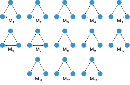
While we often regard networks to be built upon nodes joined together by edges, we may find it useful to look at smaller subgraphs instead. Rather than considering individual nodes to be the primary unit of analysis, we focused on substructures known as motifs, which for our project specifically, are triangular patterns between three separate nodes linked by edges which vary in number and direction.

Shown below is a collection of all the observed motifs analyzed for this project:

But why would we want to utilize motifs instead of nodes?

Depending on the domain of inquiry, certain motifs can emerge to become signficantly relevant in certain contexts. For instance, the first seven motifs are prevalent in social network analysis, while wedges such as the last five motifs are used when studying patterns in air traffic between cities.

Often times, we want to cluster networks to classify nodes into distinct sub-communities to either understand key characteristics about certain categories of data, or to help make future predictions regarding unseen data in the future. While much scientific inquiry has been done about clustering networks both accurately and efficiently on the level of nodes, little investigation has been done regarding clustering on a higher-order level of motifs, which is the primary motivation behind this project.

In exploring higher-order clustering of networks on the motif level, we hope that this endeavor could deepen and enrich pre-existing analyses for any domain that employs the usage of graphs.

Motif Counting

A preliminary step we must take before performing motif clustering is to count the number of occurrences of a desired motif in the given network.

For this process, we’ll utilize two data structures created while pre-processing the raw network dataset: an adjacency list for every node, which stores all the other nodes it has an edge pointing towards (named adj_list_away), and similarly another adjacency list for each node which stores all the edges that begin with other nodes and point towards it (named adj_list_in).

We then employ the following naive counting algorithm, whose general form is presented here in pseudocode:

1.) Iterate through each vertex v1 in adj_list_away
2.) Iterate through each vertex v2 which v1 points to 
    in adj_list_away
3.) Iterate through each vertex v3 which v2 points to 
    in adj_list_away
4.) Check that the number and directions of the iterated
    edges match that of the desired motif
5.) If so, record the edges amongst (v1, v2, v3) as an
    observed instance of the motif       

As shown above, our counting method maintains a computation time complexity of O(n^3) by naively iterating through each possible path of node triples in the network to check for any observed instance of the desired motif, which we aim to improve upon with our sampling method. Depending on the domain of context for any given network, certain motifs will be more prevalent than others in terms of the frequency of occurrence. For example, the number of recorded instances for each of the 13 motifs is displayed below for a network of North American city reachability by airline travel.

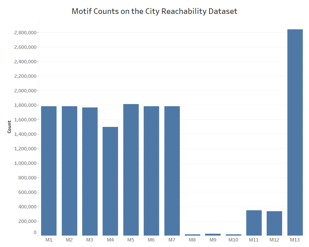
We see above that for triangular motifs, M1 through M7 all have a similar number of occurrences due to the overall density of this particular network and similarity of structure, only seemingly differing in edge direction. However, a significant outlier can be witnessed for wedges (motifs M8 to M13), for which M13 appears much more prominently than the rest.

Motif counting will ultimately act as the bottleneck in our entire pipeline to process and cluster any given network as the most time-consuming step, so later on we’ll introduce sampling techniques that will obtain a sparser subset of the graph to speed up counting while still providing a fairly accurate estimate of the optimal cluster we would obtain with the entire network. But for now, let’s move on to discussing the algorithms we’ve used to perform spectral clustering based on motif occurrences.

Spectral Clustering Algorithms

Below is a visualization of our current pipeline to count motifs and cluster network graphs based on their occurrences:

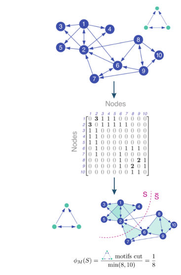
First, we count all unique instances of a target motif utilizing the counting method described earlier, which are then utilized to form the motif adjacency matrix seen in the following step. This matrix is then passed as an input into two possible spectral motif clustering algorithms presented by Austin R. Benson, David F. Gleich, and Jure Leskovec in their paper, Higher order orginazation of complex networks.

Algorithm 1

The first algorithm takes in the motif adjacency matrix, and returns a single cluster of the represented network alongside its complement, comprised by the rest of the network graph not included in the outputted cluster. Thanks to a mathematical property known as the Cheeger Inequality, this algorithm is theoretically guaranteed to find clusters which receive minimal motif conductances near the optimal (within a quadratic factor to be exact!).

For a more in-depth discussion of this algorithm and its derivation, see page 5 of the accompanying project report.

Algorithm 2

The second algorithm operates in a very similar fashion to the first by taking in a motif adjacency matrix as an input. However, unlike the first, this algorithm also takes in another parameter k, and returns k clusters instead of just a single one. The caviat however, is that this algorithm isn’t backed by the same theoretical guarantees of the Cheeger Inequality for obtaining clusters with near optimal motif conductance.

For a more in-depth discussion of this algorithm and its derivation, see page 6 of the accompanying project report.

Network Sampling

As discussed earlier, motif counting is the most time-consuming step of the pipeline which can be costly in a practical setting when computational resources are finite. Thus, our workaround is to utilize network sampling such that motif counting will only be done on a smaller subset of the original network which ideally minimizes the total runtime while still preserving as much contextual information as possible to obtain near-optimal clusters.

The sampling algorithm is outlined below:

1.) Establish a sampling threshold k
2.) Depending on the motif of interest designate 
    a "central" node p
3.) Repeatedly iterate through each edge in the 
    adjacency lists until vertex p is reached
4.) Count the number of edges n extending from vertex p 
    which are a part of an instance of the desired motif
5.) If n <= k, count all of those edges towards 
    instances of the desired motif to cluster on
6.) Otherwise, randomly sample k of the possible valid
    edges for the motif instances
7.) When forming the motif adjacency matrix for the 
    clustering algorithms, the counts of any sampled
    edges are upscaled by a factor proportional to
    the degree of the p    

The below diagram provides a simple demonstration of network sampling:

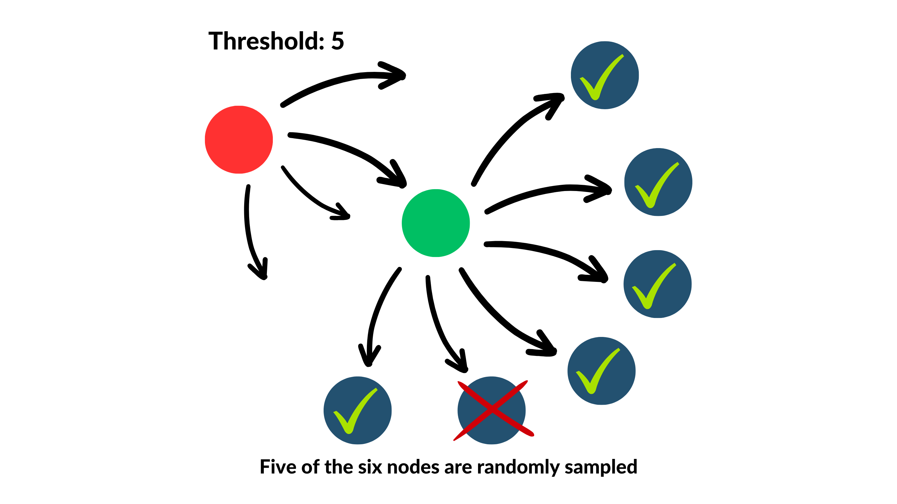
In this example, the sampling threshold is set to 5, such that if we were to sample edges from the green node to be node p (assuming they all are part of valid motifs instances), only 5 of its 6 would be selected, but their represented counts in the motif adjacency matrix would be upscaled by a calculated factor proportional to 6.

On the other hand, if instead we were to sample from the red node as p (following the same assumption), because it only has 4 edges, which is fewer than the threshold, then all of its edges would be accounted for!

Results

To gauge the effectiveness of our sampling algorithm with respect to the execution time and preserved accuracy of our motif counting and clustering pipeline, the accuracy of numerous clusters were measured from various datasets for multiple parameter combinations between the choice of motif and the value of threshold k. To examine the effects of raising the sampling threshold, we first started with the network of city reachability via airline travel introduced earlier, and calculated the accuracy of clusters computed after sampling at increasing intervals for k. These results are displayed in the following table and visualization:

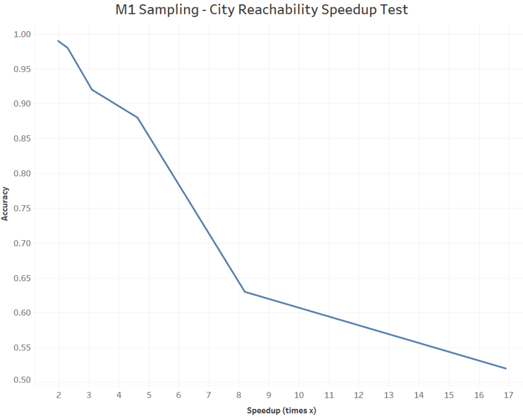
Threshold	Accuracy	Speedup
2	0.52	16.893
5	0.63	8.193
10	0.88	4.614
15	0.92	3.096
20	0.98	2.286
25	0.99	1.968

Spectral clustering was performed upon occurrences of motif M1 after sampling the graph at various values for the threshold k, which range from the interval [2, 25]. It can be seen that the largest threshold of 25 obtained a near perfect accuracy of approximately 99%, almost matching the input adjacency matrix obtained from the original graph, while executing twice as fast. Reducing the threshold size does visibly improve execution speed by a inversely proportional multiplicative factor, but at the cost of accuracy.

Rather than constraining our analysis to just one graph however, we also investigated how the density and structure of multiple networks from various domains affected the obtainable speedup possible via sampling while still hitting a benchmark accuracy. This was investigated using again the city reachability network, alongside three other graphs about Bitcoin transactions, messages between email users, and links between various pages on Wikipedia. For each network, we’ve measured the speedup of the counting and clustering pipeline for a motif prominent to each at a sampling threshold which met an accuracy of approximately 80. Again, these results are displayed in the following table and visualization:

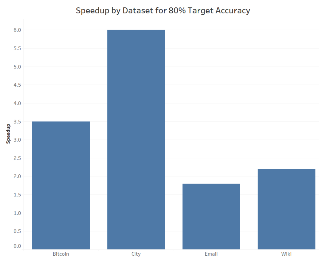
Dataset	Speedup
City	8
Wiki	2.2
Email	1.8
Bitcoin	3.5

The city reachability dataset, while sampled, reaches a remarkable 6x speedup while still obtaining 80% whereas the Wikipedia and Bitcoin graphs each manage around 2x to 3x increase in execution speed respectively. The lowest speedup obtainable was for the email network, only executing counting and clustering 1.8x times as fast, which while not necessarily an impressive magnitude at first glance, can still provide valuable practical usefulness in preserving computational resources of time and space-wise.

Discussion

From the results of our experimentation, it’s evident that a lower threshold marginally reduces the computation time at the cost of accuracy, where as a larger threshold prioritizes accuracy at a lower speedup. Although it’s best to find a Pareto-optimal sampling threshold that compromises both accuracy and speedup, the value of such a parameter inevitable varies with each network, dependent on factors such as structure and density.

Given ample time to further expand this study, we’d be eager to work with motifs of a variety of shapes, beyond that of triangular structure, alongside datasets of a much greater magnitude in size. We additionally encourage further experimentation with alternative counting methods beyond the O(n^3) naive approach that when coupled with sampling, could perhaps accelerate already existing speedups in execution. Lastly, this endeavor could be extended to empirically determine the relationship between network structure and the optimal motif for clustering, both from a context-specific and a graph theory lens.

Ultimately, the topic of motif counting and clustering of networks still remains to be a relatively new domain left with much to be researched. But nevertheless, we hope that by achieving efficient motif spectral clustering, new avenues will open for meaningful and insightful analysis of networks and scientific discovery for any academic domain of study.

References

Higher order orginazation of complex networks
Austin R. Benson, David F. Gleich, and Jure Leskovec (July 7, 2016)

Supplementary Materials for Higher-order organization of complex networks
Austin R. Benson, David F. Gleich, and Jure Leskovec (July 1, 2016)

Acknowledgments

We would like to thank Barna Saha for her mentorship and advisory throughout our endeavor, Suraj Rampure for overseeing all the administrative and logistical overhead, and finally the Halıcıoğlu Data Science Institute in making this project possible.